A Study of the Mandelbrot and Julia Sets

June 2001
This exploration is primarily concerned with a specific family of complex quadratic polynomial equations which are used to generate the Mandelbrot and Julia sets. The goal of this project is to analyze these equations from the perspective of dynamical systems theory. Amazingly, even the simplest forms of low dimensional non-linear systems generate dynamic behavior that is extremely complicated.
In general, complex dynamical systems can exhibit three distinct modes of long term behavior. For example, given a system of a given state, all trajectories of in the phase space mapping might asymptotically approach a single value. This system can be characterized by what is known as an attracting fixed point. If the system is unbounded then trajectories might escape to infinity, in which case infinity can be considered an attracting fixed point. In another scenario, the trajectories in phase space might approach a cycle of a certain frequency. This phenomenon is known as an attracting periodic orbit, or limit cycle.
However, there is a third characteristic mode of dynamic behavior that remains bounded, but is neither attracted to a fixed point or to a periodic orbit. This phenomenon is known generally as chaos. The trajectories of a chaotic system are aperiodic, meaning that the pattern never repeats itself. Chaotic systems also exhibit extreme sensitive dependence on initial conditions; thus, practical long-term prediction making is impossible. Even if only by Heisenberg’s uncertainty principle, a dynamic state of position and velocity can never be measured exactly.
Before the advent of computer technology, western thinkers assumed all dynamic behavior was either simple order, characterized by fixed points and periodic orbits, or it was completely random. The rediscovery of natural chaotic patterns by experimental mathematicians has not only demolished many antiquated misconceptions of order and randomness, but has also created an entirely new structure of reality.
The structure of this new dimension is infinitely complex, a result that stems from the fact that chaotic trajectories remain bounded and at same time are aperiodic. This infinitely complex structure is actually the limit set of a chaotic trajectory, and is often called a fractal. By mapping the flows of chaotic systems, experimenters have discovered these fractal limit sets in the form of chaotic attractors, which are dynamic maps in phase space. A few examples are the Lorenz, Rossler, and Henon attractors. Dynamic systems can also be analyzed by constructing iterative maps of equations. Of these maps, the most famous are definitely the logistic and the Mandelbrot.
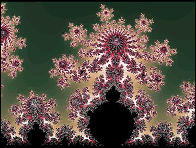
The Mandelbrot set is probably the most mysterious object in mathematics. Many aspects concerning the analysis of this structure require advanced mathematical tools and concepts. However, the Mandelbrot set is very accessible to anyone who has taken high school level mathematics. Generally speaking, the Mandelbrot is a map in the complex plane which is determined by a simple quadratic equation. Specifically, we are concerned with the following mapping:
| f c : C → C , f c (z) = z 2 + c, c,z ÎC |
Dynamic systems are characterized by a set of parameters, and a by a set of initial conditions. In the case of this complex quadratic function, the c-value is the parameter and the z-value is the initial condition, both of which are complex numbers, meaning they have two parts: one real and one imaginary. To study this equation as a dynamic system, we use an iterative process whereby we input the initial condition, compute the output, and then feed the output back into the original equation. This list of successive iterations is called the orbit of the given initial condition.
To start with, let’s consider the dynamics of f c under the initial condition of z o = 0. Obviously, for different values of c, the mapping of f c(0) will produce many different orbits. For example, if c = 0, then fc (0) remains fixed for all iterations. If c = -1, then the orbit of fc (0) is a perfect period-2 cycle. If c = i, then the orbit eventually approaches a period-2 cycle. If c = -2, then fc (0) approaches a fixed point. On the other hand, if c = 2, then the orbit of fc (0) escapes to infinity. These simple examples can easily be verified with few short calculations.
If we observe the orbits of fc (0) for all c-values, in the complex plane, we will discover a rich landscape of various forms of dynamic behavior. There are attracting fixed points, there are attracting limit cycles, there are orbits that tend to infinity, and there are orbits that are seemingly bounded and aperiodic. The Mandelbrot set is a map in the parameter plane that graphically demonstrates the behavior of fc (0) for all c-values.
To map this set using a computer, all you have to do is follow this simple algorithm. First set an upper bound N, which is the maximum number of iterations to be performed. Then, for each point c in the plane, check the first N iterates of fc (0). If | fi c (0) | > 2 for some i ≤ N, then c is not in the Mandelbrot set. On the other hand, | fi c (0) | ≤ 2 for all i ≤N, then assume c is in the Mandelbrot set and color c black. The Mandelbrot set, M, includes all c-values for which the orbit of z o = 0, under the mapping of fc , remains bounded.
| M : { c │ | f n c (0) | does not escape to infinity, c Î C } |
The c-values that escape to infinity are usually assigned a color which represents how many iterations it took for the orbit to each the upper bound N. In other words, the color of a c-value indicates how fast the orbit escapes to infinity. However, any computer mapping of the Mandelbrot is only an approximation because it is impossible to compute an infinite number of iterations. Some orbits of fc (0) escape to infinity very slowly, or after many iterations. Thus, by increasing the number of iterations, N, a more accurate picture is obtained; however, increasing the number of iterations dramatically increases the time required to compute the orbits.
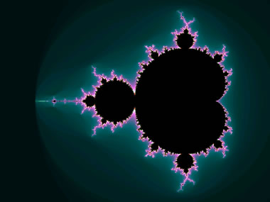
The Mandelbrot set
It can be shown that the entire Mandelbrot lies inside a disk of radius 2 centered at the origin. The escape criterion for fc (0) states that if | z | > 2, the orbit diverges toward infinity. The following is a simple proof.
If | z | > 2, then | z2 + c | ³ | z2 | - | c| > 2| z |- | c|. If | z | ³ c, then 2| z |- | c| > | z |. So if | z | > 2 and | z | ³ c, then | z2 + c| > | z |. Therefore, the sequence is continuously increasing. ٱ |
The next step is to ask, for which c-values does the orbit of fc (0) have an attracting fixed point? Let zc denote a fixed point for fc . If zc is an attracting fixed point it must satisfy the following equations.
fc (z) = z2 + c = z (the definition of a fixed point) | fc ¢(z) | = | 2z | ≤ 1 (the condition for an attracting fixed point) |
The second equation means that zc lies on or inside a circle of radius ½. On this circle | fc ¢(z) | = 1, so the fixed point zc is neutrally stable, which means that it is neither repelling nor attracting. If | fc ¢(z) | < 1, then zc is an attracting fixed point. Also, we can write z in exponential form so that z = ½ eqi . Then we can define the region of the attracting fixed points by finding an equation for the boundary that is formed by all c-values for which fc has a neutral fixed point. Using the equations above, one can easily see that c = z - z2 . Equivalently, c = x(q) = ½eqi - ¼ e2qi . This parameterized curve traces out the large central region of the Mandelbrot set. The interior of this region contains all c-values for which fc has an attracting fixed point. This region is often referred to as the main cardioid of the Mandelbrot set.
Next, consider the region of the M-set that has an attracting cycle of period 2. As mentioned above, the orbit of fc (0) has an attracting 2-period at c = -1. In fact, it can be easily proved that the region of 2-period orbits is bounded by a circle given by | c + 1 | = ¼, which is a circle of radius ¼ centered at z = -1. This region corresponds to the large bulb directly attached to the left of the main cardioid. In other words, all c-values within this bulb will generate an orbit of fc (0) that approaches a cycle of period 2.
The bulb-like regions directly attached to the main cardioid are called primary bulbs, and there are an infinite number of them. Moreover, each primary bulb consists of c-values for which fc (0) has an attracting cycle of some period p, where p is some integer. In other words, each primary bulb corresponds to a different period, and all c-values in the same primary bulb generate orbits which approach a cycle of the same period p.
The Mandelbrot set graphically depicts for which c-values the orbit of fc (0) will have an attracting fixed point (main cardioid), an attracting periodic orbit (primary bulbs), or will diverge to infinity (colored region). What about the dynamics of fc for other values of initial conditions besides zo = 0? The dynamics of the fc (z) = z2 + c vary widely for various choices of the parameter c. To analyze this system we will fix a certain value for c and compute the orbits of various possibilities of initial conditions, zo. In other words, we will check fc (z) = z2 + c for all z, given a specific c-value. This mapping lives in the dynamic plane, whereas the mapping for the Mandelbrot set lives in the parameter plane.
To obtain this dynamic map of fc (z) we use a procedure similar to the algorithm used to generate the Mandelbrot set.. First, set a maximum number of iterations, N. Then compute the orbit of each z-value. If the orbit remains bounded, color the point black, and if the orbit escapes to infinity, color the point according to how fast it reached the maximum bound of iteration. The region of z-values for which fc (z) remains bounded is known as the filled Julia set, denoted by Kc .
| Kc : { z│ f (z) = z2 + c remains bounded for a given c, z, c Î C } |
Conventionally, the set of complex numbers is usually visualized as a plane. However, it is sometimes useful in complex analysis to view the complex numbers on a sphere. Each point in the z-plane corresponds to a point on the z-sphere, with the origin located at the bottom of the sphere. The advantage is that we can interpret the top of this sphere as the point “at infinity.” The complex sphere is the set C È {∞}. To analyze the behavior of fc near infinity, use a transformation r(z) = 1/z, which switches the value of 0 with the value of ∞. In this way we can understand f c near infinity by observing
| Fc(z) = r ( f c ( r ( z ) ) ) as z goes to zero. |
It is easy to calculate that F c (z) = 2 /(1+cz 2). This means that F c (0) = 0 for all c Î C. Also, F¢(0) = 0, which means that 0 is an attracting fixed point for F c , or, equivalently ∞ is an attracting fixed point for f c . The collection of all such points that are attracted to infinity form the basin of attraction of ∞, denoted A c (∞). Naturally, A c (∞) depends on c. The boundary of A c (∞) equals the boundary of K c , the filled Julia set. This boundary forms the separatrix for the two distinct basins of attraction, i.e. those orbits that escape to infinity and those orbits that remain bounded. This boundary is called the Julia set of f c , and is denoted by J c . In general, it is not obvious how to obtain an accurate map of J c , and there are several algorithms which can be used. One algorithm that works especially well for most mappings of J c is known as the inverse iteration method. This algorithm takes advantage of the fact that f c is supersensitive on J c , which means that in any arbitrarily small neighborhood around a point z on J c , there will be some points that diverge to infinity and other points that remain bounded. This is because J c is the boundary between two competing basins of attraction. Thus, to find J c , choose any z-value and compute its “backward orbit,” or the orbit of f -1 c , which is the inverse of f c . This function is given by f-1c (z) = ± Ö (z – c).
To compute J c using this method, first choose any point z Î C. Then compute 10,000 or so points using the inverse orbit of f c . Since f -1 c (z) has two solutions, namely ± Ö (z – c), choose one of the two at random for each iteration. To map the Julia set, plot all but the first 100 iterations.
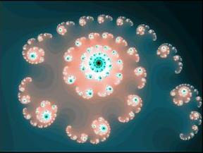
There are an infinite number of Julia sets, one for each value of c. The majority of these sets are extremely complicated. Before moving on, we will first consider two simple Julia sets. First, consider J c for c = 0. It is easy to see that f c (z) = z 2 if c = 0. Written in complex exponential form, zo = reqi . Thus, after n iterations, zn = r 2ne 2niq. Therefore, the orbit of zo escapes if and only if r > 1. Here, the radius r equals | z |, which is the norm of z = a+bi given by Ö (a 2+ b 2 ). This means that the Jo (z) escapes to infinity if zo lies outside the unit circle, which is the parameterized curve of z = reqi as q revolves form 0 to 2p. If | z | ≤ 1, then J o(z) remains bounded. Therefore, Jo = { z │| z | = 1 }. As another example, consider J-2 (z) which is the Julia set for c = -2. In this case, J-2 remains bounded only if zo lies on the interval [-2, 2]. In other words, J-2 = { z │ -2 ≤ Re(z) ≤ 2, Im(z) = 0 }.
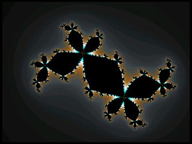
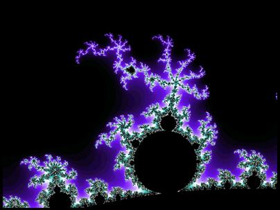
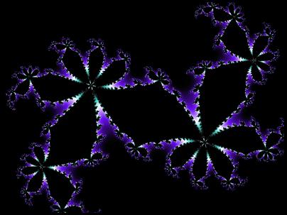
Except for the two exceptions at c = 0 and –2, all Julia sets have fractal boundaries. As mentioned above, there are an infinite variety of Julia sets. However, any given Julia set falls into one of two categories. The discovery of this fundamental dichotomy dates back to 1919 when G. Julia and P. Fatou proved that for each c-value, the Julia set is either a connected set or a Cantor set. A connected set consists of one piece whereas a Cantor set consists of an uncountably infinite set of disjoint points. If the Julia set is a Cantor set, then any arbitrarily small neighborhood around any point contains a scattered cloud of infinitely many points which do not touch
 |
 |
 |
Examples of Cantor Julia sets
The simplest example of a Cantor set is generated by the middle-thirds process. First take the line segment So = [0,1], and then remove the middle third of the segment. This produces S1 , which consists of two segments, each of which is one-third the length of the original segment. Repeat this process again and remove the middle-third of each segment in S1 , to produce S2 . At each iteration, n, there are exactly 2 n intervals and the combined length of the remaining intervals is ( 2/3 ) n . As n goes to infinity, the number of disjoint regions becomes infinite and the combined length, or measure, approaches zero. The Cantor set is the limit set of this process as n goes to infinity, C = S∞. This observation allows us to give an alternative definition for the Mandelbrot set.
If f c (0) remains bounded Þ K c is connected, and if f c (0) escapes to infinity Þ K c = J c is Cantor dust, therefore M: { c Î C | K c is connected } |
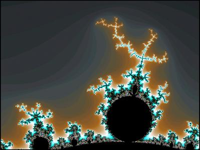
If we choose c = 0, then the corresponding Julia set is the unit circle. If we choose any other c-value which lies inside the main cardioid region, the corresponding Julia set will be a deformed circle. What happens to the filled Julia set, K c , as the value of c moves from the large cardioid into one the primary bulbs? Inside the cardioid, all orbits of f c (0) are attracted to an attracting fixed point. In the primary bulbs, all orbits of f c (0) are attracted to an attracting p-period cycle. As the c-value crosses from the cardioid into one the primary bulbs the attracting fixed point switches stability and becomes a repelling fixed point. As this happens, an attracting cycle of some period is born. Before this bifurcation, the p-period cycle was repelling.
The simplest example of this type of bifurcation occurs as the c-value moves from the large cardioid into the 2-period bulb. If we travel along the real axis, this transition occurs at c = -3/4. As the c-value crosses this point, the attracting fixed point becomes a repellor and an attracting 2-period cycle is created. For this reason, c = -3/4, is a period-doubling bifurcation point.A similar bifurcation occurs as the c-value crosses into any of the primary bulbs. The only difference is that different primary bulbs are characterized by different periods. Consider the shaped of the filled Julia sets as this transition occurs. For c-values inside the large cardioid of the Mandelbrot set, K c is congruent to some form of circular region. When the transition is made into one of the primary bulbs, the shape of the corresponding K c is pinched together at various juncture points. If the c-value has moved into a 2-period bulb, then a juncture point of K c connects two regions. If the c-value has moved into a 5-period bulb, then a juncture point of K c connects five regions.
In this way, it is easy to see that the location of the c-value in the Mandelbrot set immediately gives one an idea of what the corresponding Julia set will look like. How is it that the parameter map of the orbits of f c (0) determines the shape of the Julia set? First of all, observe that the only critical point of f c (z) = z2 + c occurs when the first derivative equals zero. In this case, f¢ c (z) = 2z, so the only critical point occurs at z = 0. By theorem, if there is an attracting periodic cycle of f c , then the critical point must “find” it. A quadratic polynomial always has infinitely many cycles; however, if there is only one critical point, then there is at most one cycle which is attracting. For this reason, the map of the only critical point, f c (0), illustrates where f c (z) will have attracting periodic orbits. Consequently, we know that if we choose any c-value from any primary bulb of the Mandelbrot, the corresponding dynamics of the filled Julia set will contain an attracting periodic cycle. The following diagram illustrates a number of primary bulbs and their periods.
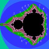
Each primary bulb in the Mandelbrot set corresponds to a certain period, call it p. The period of any given primary bulb can be determined in several ways. The analytic approach is to compute the orbit of f c (0) for a c-value that lies within the bulb. This orbit will approach a cycle of period p. Another approach is to consider the Julia set for a c-value inside a primary bulb. The period of the bulb can be determined by the filled Julia set because the critical point z = 0 determines the dynamics of K c .
As mentioned above, the filled Julia set for a c-value in a primary bulb contains a number of regions which are connected at juncture points. The number of regions connected by a single juncture point equals the period of the bulb. However, the simplest method to determine the period of a bulb requires only a visual interpretation of the Mandelbrot set. At the tip of each primary bulb, there is an antenna like structure. These antennas consist of a number of spokes which emanate from a central junction point. Amazingly, the period of a bulb attached to the main cardioid is equal to the number of spokes on the antenna attached to that bulb.
A period-4 primary bulb |
A Julia set from inside the period-4 bulb |
A period-6 primary bulb |
A Julia set from inside the period-6 bulb |
A period-16 primary bulb |
A period-21 primary bulb |
Let us now consider the periodic dynamics of K c for c-values within a primary bulb. This analysis will show that each bulb can also be characterized by a type of rotation number. The filled Julia set of a c-value from a period p bulb will consist of a number of juncture points each of which connects p regions. Each juncture point is actually a repelling fixed point of f c (z). Observe the orbit for some z that lies in one of the regions. The cycle of this orbit jumps a certain number of components in the counterclockwise direction at each iteration. Let q represent the number of regions that the orbit skips between each iteration. Since, there are exactly p regions connected by each junction point, the value q/p is type of rotation number which describes the periodic cycle of f c (z).
The most obvious method to determine the value of q/p is to compute K c , and then observe the periodic orbit. For example, if there are five regions connected at each juncture point and the orbit skips three regions between each iteration, then the rotation number is 3/5. There are also two ways to determine q/p simply by visual inspection. First, consider the Julia set inspection method. Observe that the point z = 0 lies in the largest region of K c . Then find the smallest of the remaining regions. This region is located exactly q/p revolutions about the juncture point in the counterclockwise direction. We can also determine q/p by inspecting the Mandelbrot set. Each p-period primary bulb has an antenna which consists of p spokes. For most bulbs, the shortest spoke is located q/p revolutions in the counterclockwise direction from the main spoke. Unfortunately, this last method does not work in all cases.
Now that we understand how to determine the value of the rotation numbers and what they represent, let’s observe how they are arranged. Remember, each primary bulb can be labeled with a specific rotation number. Consider the sequence of rotation numbers generated by traveling along the main cardioid in the counterclockwise direction. Amazingly, this sequence is exactly the rational numbers between zero and one. Start at the cusp, which is where the cardioid intersects with the positive real axis, and call this point zero. As we travel along the cardioid in the counterclockwise direction, we visit each bulb corresponding to rotation number q/p in exactly the same order as the rational numbers, ending at one when we arrive back at the cusp. This is truly one of the most amazing natural properties of the Mandelbrot set.
There is also an amazing pattern that been discovered which is based solely on the period numbers p. In this example, call the main cardioid the “period-1 bulb.” Also, note that the period-2 bulb is the largest primary bulb and extends to the left of the cardioid. Now, observe that the largest bulb between the period-1 and period-2 bulb is the period-3 bulb, either at the top of the bottom of the Mandelbrot set. Next, observe that the largest bulb between period-2 and period-3 is period-5. If the pattern isn’t obvious yet, consider the largest bulb between period-3 and period-5, this bulb is period-8. The sequence generated by this process is the Fibonacci sequence. If you have a nice Mandelbrot explorer you can verify that the pattern continues on. ( 1, 2, 3, 5, 8, 13, 21, 34, 55, . . . )
The intricate structure of the Mandelbrot arises because of its fractal nature. In one sense, the boundary of this set is finite; however, the length of the perimeter of this boundary is infinite. The boundary exhibits infinite complexity in that increasing the amount of magnification only brings out more and more intricate details. The only limit to how far we can explore magnifications of this boundary is the computing speed of our present technology.
Fractals are different from ordinary objects in two important ways: dimensionality and self-similarity. Firstly, consider the concept of dimension. A general definition of the dimension of a set is the minimum number of coordinates required to describe every point in the set. This is often referred to as the topological dimension. For example, a line segment is one-dimensional, a planar surface is two-dimensional, and a spherical object is three-dimensional. The topological dimension of a set is always a positive integer. However, fractals exhibit self-similarity across all scales of magnification. This feature leads to paradoxes when we try to define the topological dimension of the set. In result, the discovery of fractals has led to new definition of dimension. The similarity dimension, or fractal dimension, can be defined as follows. Suppose the set S may be subdivided into k congruent pieces, each of which may be magnified by a factor of M to yield the whole set S. Then the fractal dimension D of S is
log
(k) log
(number of pieces) |
There are several possible notions of similarity dimension such as the Hausdorff dimension, the capacity dimension, the box dimension, and the correlation dimension. In many cases, the fractal dimension of a set is not an integer, but is often some value between whole numbers. In general a fractal can be defined as a subset of Rn which is self-similar, and whose fractal dimension exceeds its topological dimension.
However these definitions of a fractal and dimension can only be rigorously applied to fractals that are simply self-similar. A few examples are the Koch Curve, the Sierpinski Triangle, and the Cantor middle-thirds set. These fractals are called affine self-similar, which means that the set S can be subdivided into k congruent subsets, each of which may be magnified by a constant factor M to yield the whole set S. In each of the above the examples the fractal dimension is a non-integer which is greater than the topological dimension.
Unlike the affine self-similar fractals, the Mandelbrot set is quasi self-similar. Magnifying any region of the boundary will produce endless self-similar details; however, the similarity is only statistical and the details on different scales are never exactly the same. This type of statistical self-similarity can be found in all forms of nature. Since the Mandelbrot is not affine self-similar our regular definition of similarity dimension makes no sense. If we we’re to speak generally, we could say that the Mandelbrot set has a dimension of 2. This is because the entire set is contained in a disk which has a dimension of 2. The topological dimension of the Mandelbrot is 1. This is because the boundary has an empty interior, so the dimension must be less than 2, and is therefore 1. In any case, all of our present conceptions of dimensionality and fractals are practical working definitions and are by no means rigorously defined.
The Mandelbrot set can also be mapped in higher dimensions. The classic Mandelbrot set is a map in the complex plane. Each coordinate in the plane is essentially 2 dimensional because a complex number, z, has two parts and is written z = a + ib. Complex numbers have one part which is real and a second part which we call imaginary. To introduce Mandelbrot sets in higher dimensions we must use quaternions. Quaternion numbers are an extension of complex numbers, which have four parts instead of two. A quaternion Q equals a + ib + jc + kd, where the coefficient a, b, c, and d are real numbers. Operations such as addition and multiplication can be performed on quaternions, but multiplication is not commutative. Quaternions satisfy the following rules:
i2 = j2 = k2 = -1 ij = -ji = k jk = -kj = i ki = -ik = j |
The normal Mandelbrot and Julia formulas can be extended to use quaternions instead of complex numbers. Complex numbers can be displayed on a plane because they have two parts. A quaternion Mandelbrot set mapping requires four dimensions to be viewed because each value has four parts. In addition, each c-value of the four-dimensional Mandelbrot corresponds to a specific four-dimensional Julia set.
Presently, we are unable to visualize these higher dimensional objects directly. One method of analyzing a 4D quaternion object is to "take slices." If we take slices of a 3D object we will get a bunch of 2D objects. If we take slices of a 4D object we will get a bunch of 3D objects. To get an idea of what the fourth-dimensional object looks like, take all the slices and create an animation of the 3D objects as the slice moves through the quaternion set. This method utilizes time as the fourth dimension, which is exactly what Einstein did to describe the four-dimensional space-time continuum.
 |
 |
|
 |
 |
|
 |
 |
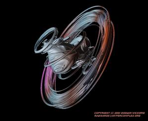
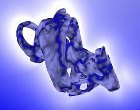
Some examples of 3D slices of Quaternion fractals
 |
 |
|
 |
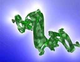 |
Some more examples of 3D slices of Quaternion fractals
What if our life is an animation of 3D slices taken from a 4D continuum? My interpretation of this question goes something like this. If there is only one space-time continuum, then everything is determined and there is no free-will. This may be the case, however, I think there is a large amount of evidence to the contrary. There are only two other possibilities. The first possibility is that there are an infinite number of continuums, an idea similar to the Many-Worlds Interpretation of Quantum Theory. The other possibility is that only the moment really exists, and the past and the future only exist as potential probabilities.
It may be that these three possibilities do not contradict each other, in which case reality would have to be infinite-dimensional. For example, perhaps our 4D continuum is only one slice of a 5D continuum, then there are actually an infinite number of 4D continuums. Maybe the 5D dimensional continuum is only one slice of an even higher dimensional continuum, and so forth and so on to infinity. As another example, consider that the many moments that we experience in time are actually lower dimensional slices of one higher dimensional moment. In other words, if we could see a higher dimensional continuum without having to take lower dimensional slices, we could see all the past and all the future at one glance. Indeed, we create time by taking these slices. In the case of quaternion fractals, if we could see in four dimensions we wouldn’t need to create animations of lower dimensional slices. The implications of these examples suggest that there is only one infinite dimensional moment which is eternally beyond all finite dimensional continuums, of which there are infinitely many. At the same time, all the past and future exist only as potential probabilities created by slicing the infinite dimensional moment of eternal now in an infinite number of ways.
The exploration of these higher dimensional fractal objects represents the newest frontier of mathematics as well as computer technology. Amazingly, these hyperspatial images can be generated simply by using the basic quadratic equation f c (z) = z2 + c. As we have seen, this simple equation can be used to demonstrate almost all important aspects of dynamical systems theory. We have encountered fixed points, periodic orbits, sensitive dependence on initial conditions, self-similarity, fractals, dimension, Cantor sets, and basins of attraction.
The maps of this quadratic equation are not necessarily chaotic attractors in the normal sense of the term. In general, a chaotic attractor is the limit set of an aperiodic trajectory. This region remains bounded, but the pattern never repeats so the attractor will always have a fractal structure. The dynamic mapping of f c (z) = z2 + c, for a fixed c, is the Julia set. The filled black region represents the z-values that behave orderly, either as periodic cycles or fixed points. The colored region represents the z-values that will escape to infinity. The Julia set, J c , is the boundary between these two competing basins of attraction. Remember that the boundary of Julia set is only an approximation, which is limited by the number of iterations we calculate to see if the z-value escapes to infinity. If we could take an infinite number of iterations, which we can’t, the boundary of J c would consist of all z-values which have bounded, aperiodic orbits. Thus, J c is a map of all z-values which have a chaotic limit set.
In addition, it can be proved that for any c-value, the repelling periodic points of f c (z) are dense in the Julia set, J c . It can also be shown that f c (z) is supersensitive at any point in J c . This has already been discussed in the segment concerning the Inverse Iteration Method for finding the Julia set. Consequently, if we analyze the dynamics of f c (z) by reversing the flow of time, the Julia set is actually the limit set of chaotic orbits, and thus can be thought of as some sort of chaotic attractor. If time is flowing in the conventional forward direction, the Julia set is something like a chaotic repellor.
In closing, let us make sure we clearly understand that the Mandelbrot and Julia sets are different ways of looking at the same thing. For the Mandelbrot, we hold z constant at 0 and check all c-values. For the Julia set, we hold c constant and check all z-values. Perhaps with more sophisticated computer graphics technology we will be able to analyze the mapping of f c (z) by modulating both the parameter values and the initial condition values at the same time. In any case, it is certain that the frontier of Chaos Theory is a field of infinite fractal possibilities.

Sources
Abraham, Ralph. Dynamics – The Geometry of Behavior; Part 2: Chaotic Behavior. Aerial Press, Inc. Santa Cruz. 1983.
Devaney, Robert. A First Course in Chaotic Dynamical Systems. Addison-Wesley Publishing Company, Inc. 1992.
Devany, Robert and Linda Keen, editors. Chaos and Fractals. American Mathematical Society. 1988.
Peitgen, Heintz-Otto and Dietmar Saupe, editors. The Science of Fractal Images. Springer-Verlag. 1988.
Strogatz, Steven H. Nonlineral Dynamics and Chaos. Perseus Publishing. 1994.
· images of two-dimensional fractals were created using a program named Xaos.
· images of quaternion fractals were taken from the following website, http://www.hypercomplex.org/quats.htm